高斯过程 是一种常用的监督学习 方法,可以用于解决回归和分类问题。
预测对观察结果进行了插值
预测的结果是概率形式的
通用性:可以指定不同的核函数(kernels)形式
高斯过程模型的确定包括:
它们不是稀疏的,即它们使用整个样本/特征信息来执行预测
高维空间模型会失效,高维也就是指特征的数量超过几十个
值得注意的是,高斯过程模型的优势主要体现在处理非线性 和小数据 问题上。
参考资料:https://scikit-learn.org/stable/modules/gaussian_process.html
若一个随机变量X X X μ \mu μ σ 2 \sigma ^2 σ 2 X ∼ N ( μ , σ ) X \sim N(\mu, \sigma) X ∼ N ( μ , σ )
f ( x ) = 1 σ 2 π e − ( x − μ ) 2 2 σ 2 f(x) = \frac{1}{\sigma \sqrt{2\pi}}e^{-\frac{(x-\mu)^2}{2\sigma^2}}
f ( x ) = σ 2 π 1 e − 2 σ 2 ( x − μ ) 2
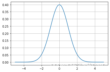
对于均值为0,方差为1的高斯分布可以画出其函数图像:
1
2
3
4
5
6
7
import matplotlib.pyplot as pltimport numpy as npx = np.linspace(-5 , 5 , 10000 ) y = 1.0 /np.sqrt(2.0 *np.pi)*np.exp(-1.0 *np.power(x, 2 )/2.0 ) plt.plot(x, y) plt.grid()
对于任意维度的随机变量X ( x 1 , x 2 , ⋯ , x n ) X(x_1, x_2, \cdots, x_n) X ( x 1 , x 2 , ⋯ , x n ) X ∼ N ( μ , ∑ ) X\sim N(\mu, \sum) X ∼ N ( μ , ∑ ) ∑ \sum ∑
f ( X ) = 1 ( 2 π ) n ∣ ∑ ∣ e − 1 2 ( X − μ ) T ∑ − 1 ( X − μ ) f(X) = \frac{1}{\sqrt{(2\pi)^n|\sum|}}e^{-\frac{1}{2}(X-\mu)^T\sum ^{-1}(X-\mu)}
f ( X ) = ( 2 π ) n ∣ ∑ ∣ 1 e − 2 1 ( X − μ ) T ∑ − 1 ( X − μ )
其中协方差矩阵的形式为:
[ σ ( x 1 , x 1 ) ⋯ σ ( x 1 , x n ) ⋮ ⋱ ⋮ σ ( x n , x 1 ) ⋯ σ ( x n , x n ) ] \begin{bmatrix}
\sigma(x_1, x_1) & \cdots & \sigma(x_1,x_n) \\
\vdots & \ddots & \vdots \\
\sigma(x_n, x_1) & \cdots & \sigma(x_n, x_n)
\end{bmatrix}
⎣ ⎢ ⎡ σ ( x 1 , x 1 ) ⋮ σ ( x n , x 1 ) ⋯ ⋱ ⋯ σ ( x 1 , x n ) ⋮ σ ( x n , x n ) ⎦ ⎥ ⎤
其中
σ ( x i , x j ) = ∑ k = 1 c ( x i k − x i ˉ ) ( x j k − x j ˉ ) c − 1 \sigma(x_i, x_j) = \frac{\sum^{c}_{k=1}(x_i^k-\bar{x_i})(x_j^{k}-\bar{x_j})}{c-1}
σ ( x i , x j ) = c − 1 ∑ k = 1 c ( x i k − x i ˉ ) ( x j k − x j ˉ )
其中c代表样本总数,协方差矩阵反映了不同变量之间的相关性大小,如果各个变量之间不相关,那么该矩阵为单位阵。关于多元高斯分布的一个重要性质就是:多元高斯分布的条件分布同样符合高斯分布。
参考资料:https://zhuanlan.zhihu.com/p/518236536
顾名思义,高斯过程回归就是通过高斯过程来求解回归问题,回归是指通过适当的建模来拟合一组自变量X X X y y y
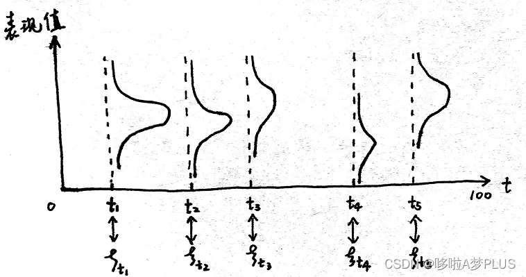
将多元高斯分布推广到连续域上的无限维高斯分布,就得到了高斯过程。如下图所示,在时域T T T t i t_i t i t i ∼ N ( μ i , σ i ) t_i \sim N(\mu _i, \sigma _i) t i ∼ N ( μ i , σ i ) T T T
T ( t 1 , t 2 , ⋯ , t n ) ∼ N ( μ ( t ) , ∑ ( t i , t j ) ) T(t_1, t_2, \cdots,t_n)\sim N(\mu(t), \sum(t_i, t_j))
T ( t 1 , t 2 , ⋯ , t n ) ∼ N ( μ ( t ) , ∑ ( t i , t j ) )
其中每个时刻的均值用一个均值函数刻画,两个不同时刻之间的相关性用一个协方差函数刻画。
因此我们只需要两个因素来确定一个高斯过程:
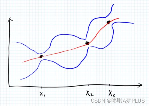
高斯过程回归的是通过有限的高维数据来拟合出相应的高斯过程,从而来预测任意随机变量下的函数值。具体而言,对于一组随机变量X 1 , X 2 , ⋯ , X n X_1, X_2, \cdots, X_n X 1 , X 2 , ⋯ , X n y 1 , y 2 , ⋯ y n y_1, y_2, \cdots y_n y 1 , y 2 , ⋯ y n
[ X 1 , X 2 , ⋯ , X n ] ∼ N ( y 1 , y 2 , ⋯ , y n , ∑ ) [X_1, X_2, \cdots, X_n]\sim N(y_1, y_2, \cdots, y_n,\sum)
[ X 1 , X 2 , ⋯ , X n ] ∼ N ( y 1 , y 2 , ⋯ , y n , ∑ )
这其中的问题是需要确定协方差矩阵,它反映了不同采样点之间的相似性大小,合法的协方差矩阵要求是半正定的,因此这里我们需要指定相应的核函数来度量这一相似性,sklearn中提供了很多的核函数,后面介绍。确定了协方差矩阵之后,我们就能根据已有的数据确定变量空间中的无限维高斯分布,并且相应地能够确定任意采样点处的条件高斯分布,即是相应的概率分布 ,如下图所示:
前面已经说明,核函数的作用是描述不同采样点之间的相似性大小,sklearn中内置了很多核函数,如下图所示:
除了sklearn中提供的核函数之外,也可以自定义核函数。
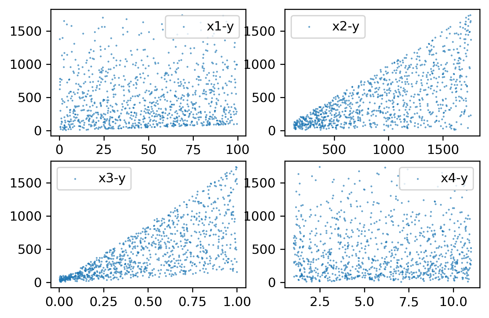
这里我们利用 sklearn.datasets.make_friedman2 生成初始数据,friedman2 生成输入数据是一个 n_sample x 4维的矩阵,下面是其调用及可视化。
1
2
3
4
5
6
7
8
9
10
11
12
13
14
15
16
17
18
19
20
21
from sklearn.datasets import make_friedman2import matplotlib.pyplot as pltX, y = make_friedman2(n_samples=1000 , noise=0.1 , random_state=10 ) plt.figure(dpi=300 ) ax1 = plt.subplot(221 ) ax1.scatter(X[:, 0 ], y, label='x1-y' , s=0.1 ) ax1.legend() ax1 = plt.subplot(222 ) ax1.scatter(X[:, 1 ], y, label='x2-y' , s=0.1 ) ax1.legend() ax1 = plt.subplot(223 ) ax1.scatter(X[:, 2 ], y, label='x3-y' , s=0.1 ) ax1.legend() ax1 = plt.subplot(224 ) ax1.scatter(X[:, 3 ], y, label='x4-y' , s=0.1 ) ax1.legend()
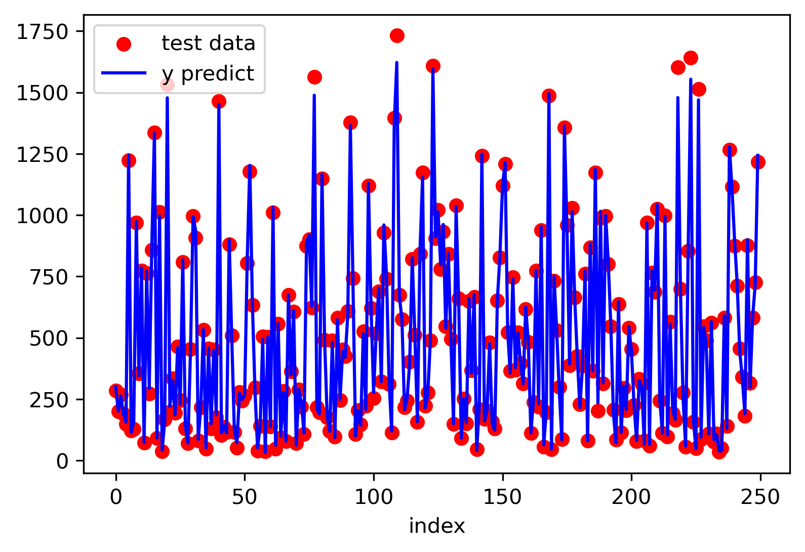
1
2
3
4
5
6
7
8
9
10
11
12
13
14
15
16
17
18
19
20
21
22
23
24
25
from sklearn.datasets import make_friedman2from sklearn.model_selection import train_test_splitfrom sklearn.gaussian_process import GaussianProcessRegressorfrom sklearn.gaussian_process.kernels import RBF, Sum, WhiteKernelimport matplotlib.pyplot as pltX, y = make_friedman2(n_samples=1000 , noise=0.1 , random_state=10 ) X_train, X_test, y_train, y_test = train_test_split(X, y, test_size=0.25 , random_state=36 ) model_kernel = Sum(RBF([100 , 1500 , 1 , 10 ], length_scale_bounds='fixed' ), WhiteKernel(0.1 , noise_level_bounds='fixed' )) model_gpr = GaussianProcessRegressor(kernel=model_kernel) model_gpr.fit(X_train, y_train) print (model_gpr.score(X_test, y_test))y_mean, y_std = model_gpr.predict(X_test, return_std=True ) plot_x = [i for i in range (X_test.shape[0 ])] plt.figure(dpi=300 ) plt.scatter(plot_x, y_test, color='red' , label='test data' ) plt.plot(plot_x, y_mean, color='blue' , label='y predict' ) plt.legend()
x 1 , x 2 , x 3 , x 4 x_1,x_2,x_3,x_4 x 1 , x 2 , x 3 , x 4 0.99 。
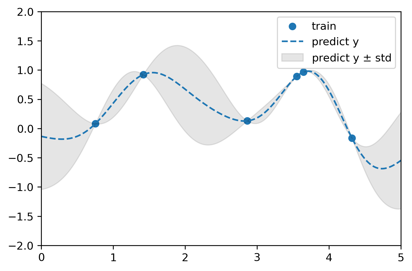
1
2
3
4
5
6
7
8
9
10
11
12
13
14
15
16
17
18
19
20
21
22
from sklearn.datasets import make_friedman2from sklearn.model_selection import train_test_splitfrom sklearn.gaussian_process import GaussianProcessRegressorfrom sklearn.gaussian_process.kernels import DotProduct, RBF, Sum, Matern, PairwiseKernelimport matplotlib.pyplot as pltimport numpy as npx_train = np.random.uniform(0 , 5 , 6 ).reshape(-1 , 1 ) y_train = np.sin(np.power(x_train-2.5 , 2 )) model_kernel = RBF(length_scale=1.0 , length_scale_bounds=(1e-1 , 10.0 )) model_gpr = GaussianProcessRegressor(kernel=model_kernel) model_gpr.fit(x_train, y_train) plot_x = np.linspace(0 , 5 , 10000 ).reshape(-1 , 1 ) y_mean, y_std = model_gpr.predict(plot_x, return_std=True ) plt.figure(dpi=300 ) plt.xlim([0 , 5.0 ]) plt.ylim([-2.0 , 2.0 ]) plt.scatter(x_train, y_train, label="train" ) plt.plot(plot_x[:, 0 ], y_mean, '--' , label='predict y' ) plt.fill_between(plot_x[:, 0 ], y_mean-y_std, y_mean+y_std, color='black' , alpha=0.1 , label=r"predict y $\pm$ std" ) plt.legend()
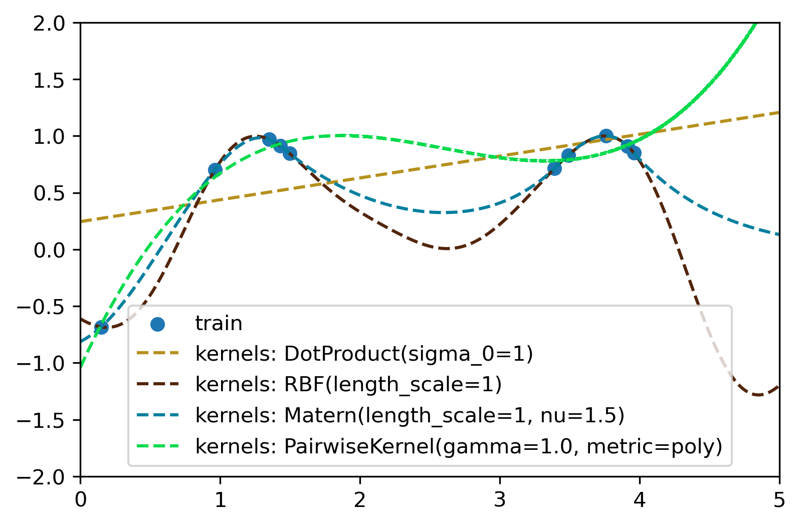
对于以上c中的数据,这里用了四种不同的核函数来拟合,如下为代码和拟合结果。
1
2
3
4
5
6
7
8
9
10
11
12
13
14
15
16
17
18
19
20
21
22
23
24
25
26
27
from sklearn.datasets import make_friedman2from sklearn.model_selection import train_test_splitfrom sklearn.gaussian_process import GaussianProcessRegressorfrom sklearn.gaussian_process.kernels import DotProduct, RBF, Matern, PairwiseKernelimport matplotlib.pyplot as pltimport numpy as npx_train = np.random.uniform(0 , 5 , 10 ).reshape(-1 , 1 ) y_train = np.sin(np.power(x_train-2.5 , 2 )) model_k1 = DotProduct(sigma_0=1 , sigma_0_bounds=(1e-1 , 10.0 )) model_k2 = RBF(length_scale=1.0 , length_scale_bounds=(1e-1 , 10.0 )) model_k3 = Matern(length_scale=1.0 , length_scale_bounds=(1e-1 , 10.0 ), nu=1.5 ) model_k4 = PairwiseKernel(gamma=1.0 , gamma_bounds=(1e-1 , 10 ), metric='poly' ) plt.figure(dpi=300 ) plt.xlim([0 , 5.0 ]) plt.ylim([-2.0 , 2.0 ]) plt.scatter(x_train, y_train, label="train" ) plot_x = np.linspace(0 , 5 , 10000 ).reshape(-1 , 1 ) for model_kernel in [model_k1, model_k2, model_k3, model_k4]: model_gpr = GaussianProcessRegressor(kernel=model_kernel) model_gpr.fit(x_train, y_train) y_mean = model_gpr.predict(plot_x) plt.plot(plot_x[:, 0 ], y_mean, '--' , color=(np.random.random(), np.random.random(), np.random.random()), label='kernels: {}' .format (model_kernel.__str__())) plt.legend()